Maricopa Housing: Dashboard + Price Predictor
Two-part Streamlit project on Maricopa County, Arizona residential property sales using public Assessor data. An interactive dashboard for exploration, plus an end-to-end ML pipeline that predicts sale price (Random Forest: 0.846 R², 13.14% MAPE on 91k test set).
Overview
A weekend dive into Maricopa County, Arizona’s residential real-estate data. Two complementary Streamlit apps share the same data pipeline: one explores the market through interactive charts, the other predicts the sale price of any property from the Assessor’s feature set. Built on the public Maricopa County Assessor R116 residential master extract.
Why two apps
The Maricopa Assessor publishes a rich pipe-delimited dump of every residential sale: 24 columns, no header row, decades of history. I wanted to do two different things with it, so I built two different Streamlit apps that share an ingestion script.
- Stats Dashboard for the question: what does the Maricopa market actually look like, by year, geography, and property class?
- Price Predictor for the question: given this property’s features, what should it sell for?
Same Parquet file feeds both. Clean separation of read-only exploration from predictive modeling.
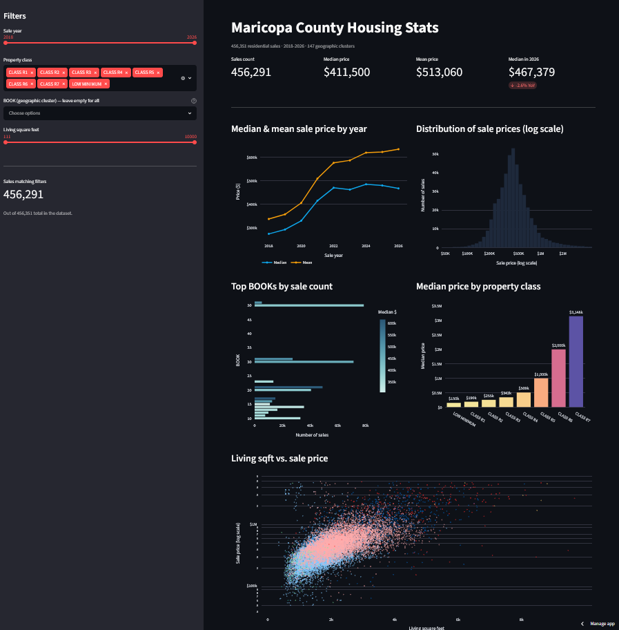
Part 1: Stats Dashboard
The exploratory side. The user picks year ranges, geography (Assessor BOOKs, which are 3-digit geographic clusters that stand in for ZIP since address columns weren’t shipped), and property class (R1 through R7), and the dashboard reflows:
- Sale-price trends across 2018 to 2026.
- Geographic comparison across BOOKs.
- Property-class distributions and medians.
- Interactive Sqft vs. price scatter (sampled, filterable).
- Quick stat cards: median, mean, count, year-over-year change.
Live: spadida-maricopa-housing-stats.streamlit.app
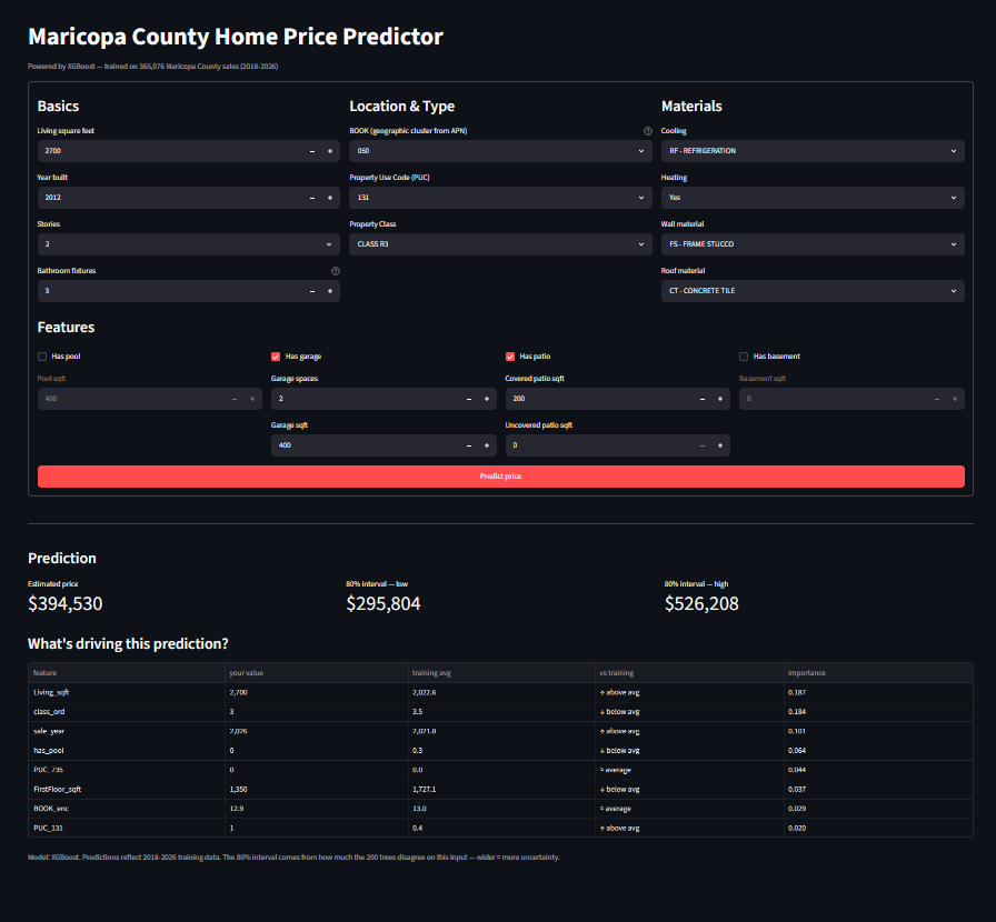
Part 2: Price Predictor
The ML side. The pipeline runs end to end: raw Assessor file in, trained model out. Ingestion filters the dump to clean residential sales and writes a Parquet snapshot. Feature engineering follows, with categorical cleanup, log-transforming the target, and dropping the columns that turned out to be empty or noisy. Two baselines (OLS and Ridge regression) set the floor, then two tree-based models (Random Forest and XGBoost) compete for the top spot. The Streamlit app loads the winning artifact at startup, takes property attributes from the user, and returns a sale-price estimate.
Live: spadida-maricopa-housing-predictor.streamlit.app
Model performance
Test set of 91,269 sales, log-transformed target:
| Model | log MAE | log R² | $ MAE | MAPE |
|---|---|---|---|---|
| Baseline (predict mean) | 0.4040 | 0.000 | $216,089 | 42.83% |
| OLS | 0.1921 | 0.705 | $111,234 | 20.14% |
| Ridge (α=1.0) | 0.1921 | 0.705 | $111,232 | 20.14% |
| Random Forest | 0.1226 | 0.846 | $73,771 | 13.14% |
| XGBoost | 0.1330 | 0.833 | $79,649 | 13.89% |
Random Forest wins on every metric, though XGBoost is close enough that the deployed artifact tradeoff is real (RF is hundreds of MB, XGBoost is much smaller, with a 1-percentage-point accuracy hit).
Notes on the data
The Assessor’s delivered file is pipe-delimited, 24 columns, no header row. A few gotchas worth knowing if you do similar work:
SALE_DATEships ISOYYYY-MM-DDeven though the legend claimsMM/DD/YYYY. Trust the data, not the docs.- Sale prices below $50K (quit-claim deeds, intra-family transfers) and above $5M (luxury outliers) are filtered out to keep the model on the central distribution.
RoofStyleis 100% empty in this extract. Dropped.- BOOK (first 3 digits of APN) substitutes for ZIP since address columns weren’t shipped.
Stack
Python, Pandas, scikit-learn, XGBoost, Streamlit, Parquet. Trained locally, deployed on Streamlit Community Cloud, both apps free to access.